The new Github repository OpenGovernmentVienna has already been created including a very nice addition by Christian.
The script executes the following steps:
- Download Vienna map including district boundaries from http://data.wien.gv.at.
- Download population and district size from https://www.wien.gv.at/statistik, calculate population density.
- Plot Vienna map coloured by population density.
library(rgdal)
library(rgeos)
library(XML)
library(RCurl)

download.vienna.bydistrict <- function(tablename, skip.row = 3) {
    baseurl <- "https://www.wien.gv.at/statistik"
    popurl <- sprintf("%s/%s.html", baseurl, tablename)

    poptable <- readHTMLTable(getURL(popurl))[[1]]
    poptable <- poptable[-c(1:skip.row), ]
    poptable <- poptable[, -1]
    row.names(poptable) <- NULL
    poptable <- sapply(poptable, function(x) gsub(".", "", x, fixed = TRUE))
    poptable <- gsub(",", ".", poptable, fixed = TRUE)
    poptable <- matrix(as.numeric(poptable), nrow = nrow(poptable))
    poptable
}

# Download Data Shape Data District Boundaries
mapdata <- "http://data.wien.gv.at/daten/geo?service=WFS&request=GetFeature&version=1.1.0&typeName=ogdwien:BEZIRKSGRENZEOGD&srsName=EPSG:4326&outputFormat=shape-zip"

dir.create("data", showWarnings = FALSE)
destfile <- "data/BEZIRKSGRENZEOGD.zip"
download.file(mapdata, destfile = destfile)
unzip(destfile, exdir = "data/BEZIRKSGRENZEOGD")
file.remove(destfile)
## [1] TRUE# Read District Boundaries
wmap <- readOGR("data/BEZIRKSGRENZEOGD", layer="BEZIRKSGRENZEOGDPolygon") ## OGR data source with driver: ESRI Shapefile
## Source: "data/BEZIRKSGRENZEOGD", layer: "BEZIRKSGRENZEOGDPolygon"
## with 23 features
## It has 15 fields# Download Population per district
distpop <- download.vienna.bydistrict("bevoelkerung/tabellen/bevoelkerung-alter-geschl-bez")
distpopsum <- rowSums(as.matrix(distpop))
# Download Size of Each district
distsize <- download.vienna.bydistrict("lebensraum/tabellen/nutzungsklassen-bez", skip.row = 2)
distsizekm2 <- distsize[, 1] / 100
wd <- data.frame(distpopsum / distsizekm2)
centroids <- gCentroid(wmap, byid=TRUE)
colfunc <- colorRampPalette(c("lightblue", "darkred"))
colnames(wd) <- "inh"
wd$district <- seq(1,23)
anstieg_pop <- wd$district[order(wd$inh)]
colsort <- colfunc(23)[order(anstieg_pop)]
layout(matrix(c(1,2), byrow = TRUE),height=c(1.3, 0.7))
par(mar=c(0,0,0,0))
plot(wmap,col=colsort[wmap$BEZNR])
text(as.character(wmap$BEZ_RZ), x = centroids@coords[,1], y = centroids@coords[,2],cex=0.8)
par(mar=c(3,4,4,2),mgp=c(2,0.7,0))
barplot(wd$inh,main="Population Density Vienna 2014",yaxt="n",col=colsort,xlab="District",beside=T, ylab=expression(paste("1.000 Inhabitants km"^-2)),names.arg=as.roman(wd$district),las=2)
axis(2,labels=c("0","5","10","15","20"),at=c(0,5000,10000,15000,20000),las=1)
abline(h=c(5000,10000,15000,20000),lty=2)
legend("topright",pch=c(15,15),col=c("darkred","lightblue"),c("high","low"),bg="white") 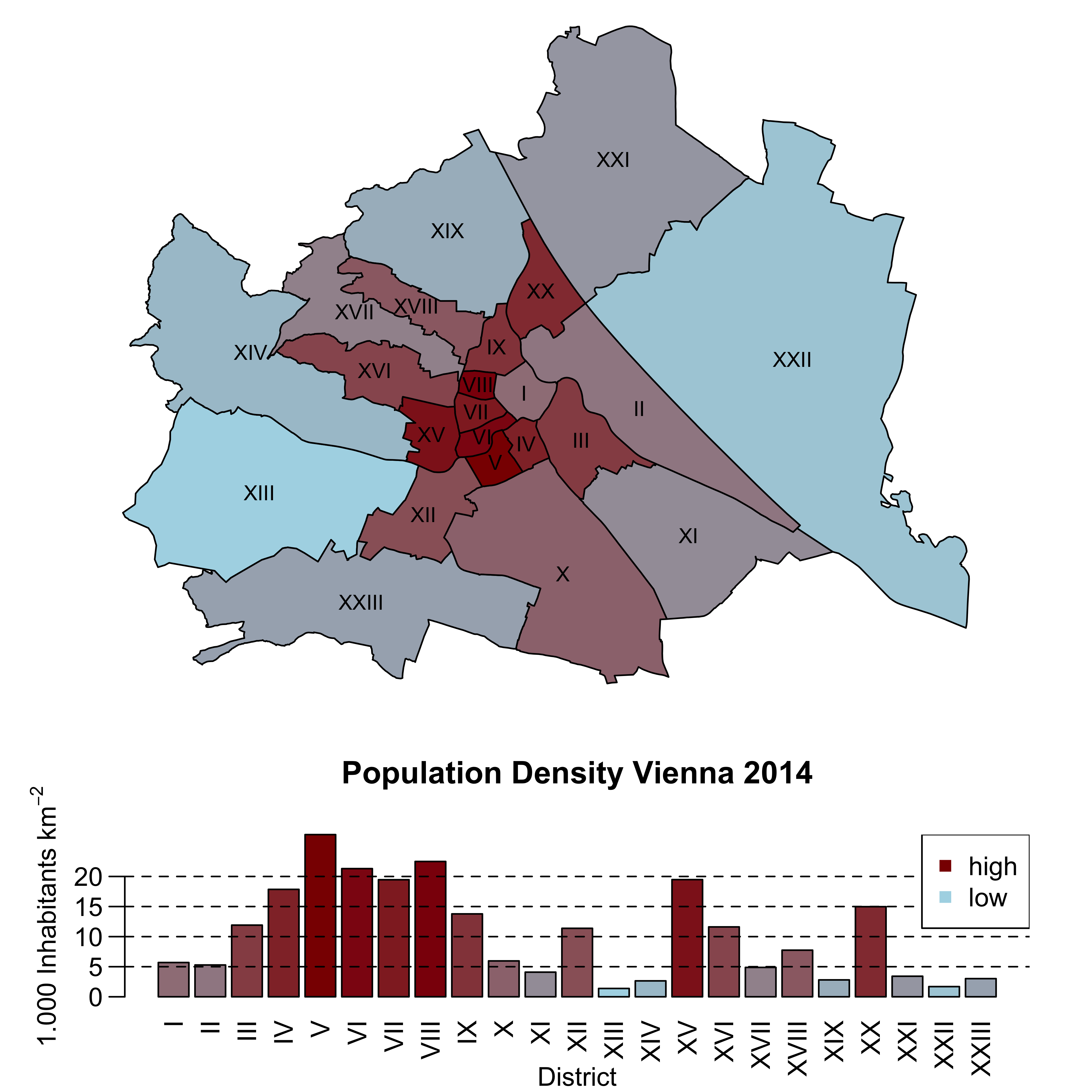
Authors: Christian Brandstaetter with small additions by Mario Annau