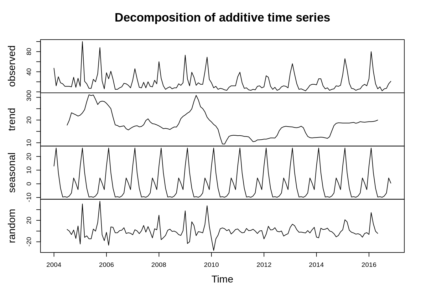
The time series can be decomposed into three components: seasonal, trend-cycle and a residual component.
\[y_t = S_t + T_t + E_t\]
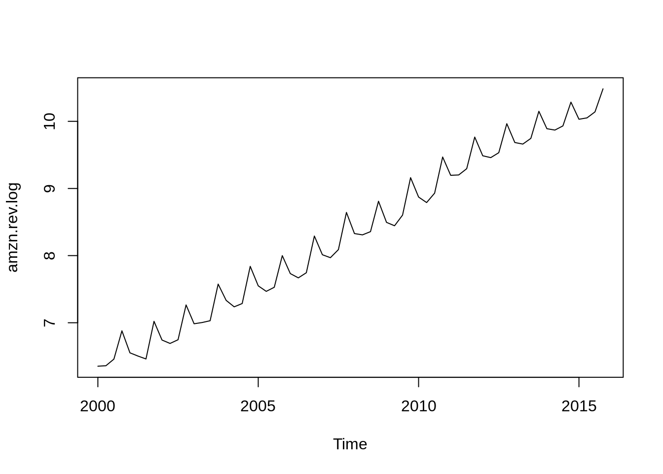
If seasonal component depends on absolute level of time series we can also use a multiplicative model
\[y_t = S_t \times T_t \times E_t\]
By taking the logarithm the additive model can be used.
dat.ts.decomp <-decompose(dat.ts, type ="additive")plot(dat.ts.decomp)
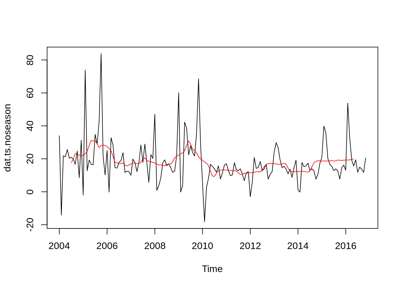
dat.ts.noseason <- dat.ts - dat.ts.decomp$seasonalplot(dat.ts.noseason)lines(dat.ts.decomp$trend, col ="red")
\[ARIMA(p,d,q)\] models can be used and are specified as \[\dots\]
(p, d, q) are the AR order, the degree of differencing, and the MA order.
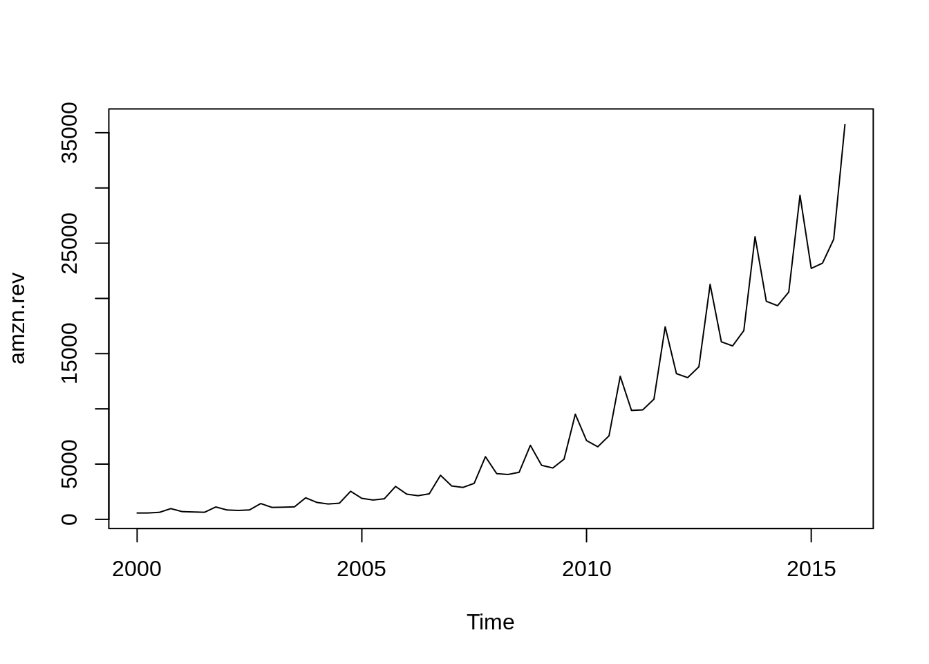
First we can check if timeseries is stationary. If not clear on plot or unsure, we can use the Augmented Dickey–Fuller Test or Kwiatkowski-Phillips-Schmidt-Shin (KPSS) test
tseries::adf.test(dat.ts, alternative ="stationary")
Warning in tseries::adf.test(dat.ts, alternative = "stationary"): p-value
smaller than printed p-value
    Augmented Dickey-Fuller Test

data:  dat.ts
Dickey-Fuller = -6.2372, Lag order = 5, p-value = 0.01
alternative hypothesis: stationary
tseries::kpss.test(dat.ts)
Warning in tseries::kpss.test(dat.ts): p-value greater than printed p-value
    KPSS Test for Level Stationarity

data:  dat.ts
KPSS Level = 0.27746, Truncation lag parameter = 4, p-value = 0.1
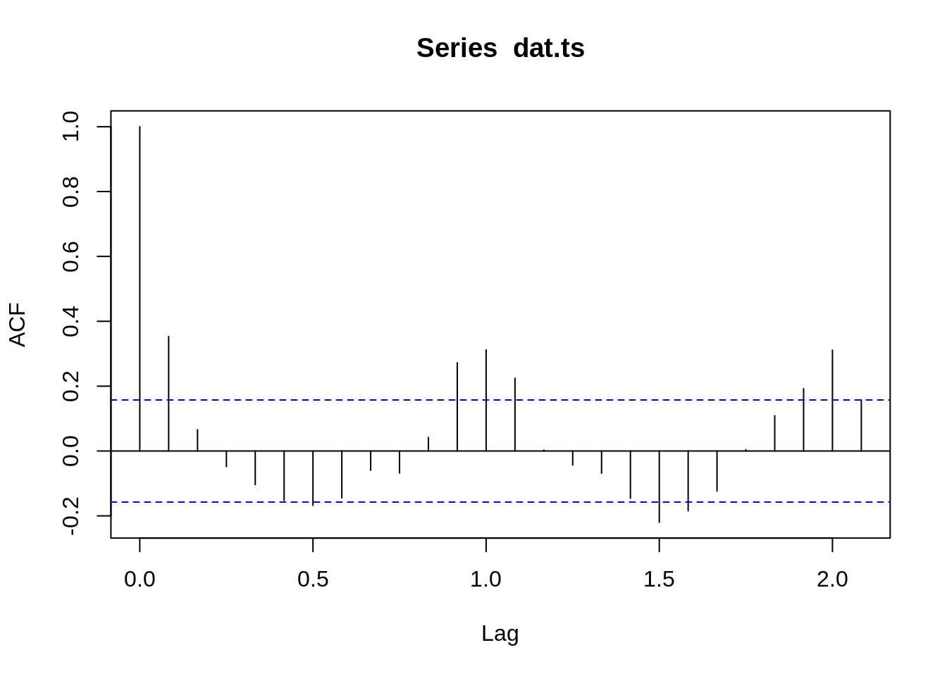
Since no differencing is required, we set \[d=0\] and check the acf and pacf plots
acf(dat.ts, lag.max =25)
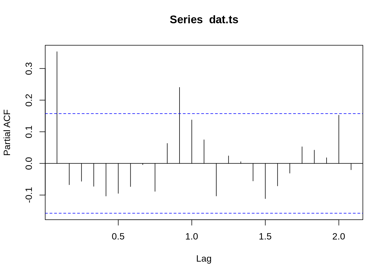
pacf(dat.ts, lag.max =25)
The acf plots suggests a second order autoregressive process, we thus set \[p=2\]. Let’s check the current model now:
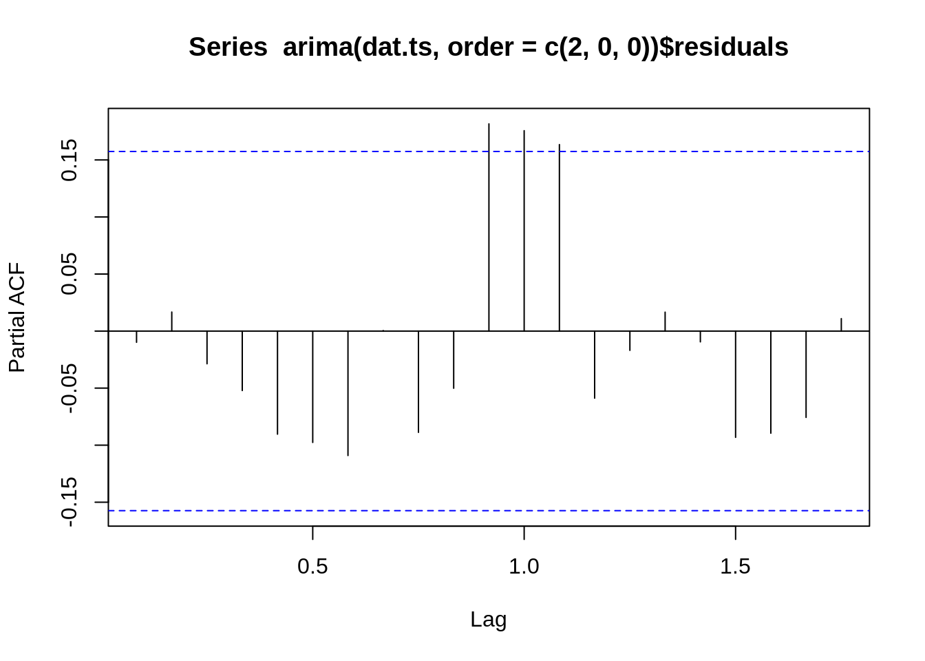
pacf(arima(dat.ts, order=c(2, 0, 0))$residuals)
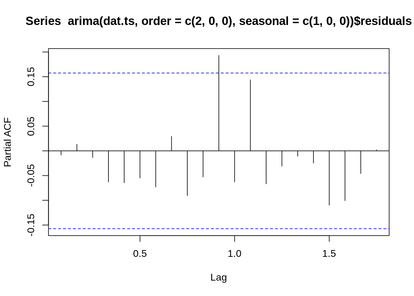
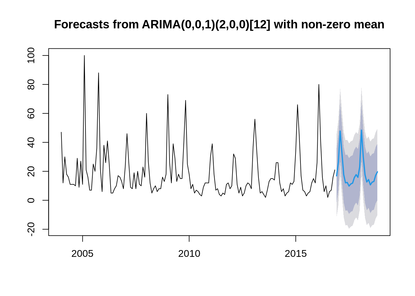
Ups - the pacf plot shows that there is still a seasonal pattern left. We try it with a seasonal order AR of \[p=1\]